Tutorial

We will be using the Iris dataset for this tutorial. First we create the dataset we will be working with, by declaring a class inheriting from Dataset which will define how we load our training and prediction data. Scikit-learn comes with handy Dataset loading utilities, so we will be using their load_iris() data loader function

>>> from sklearn.datasets import load_iris
>>> from ml_tooling.data import Dataset
>>> import pandas as pd
>>> import numpy as np

>>> class IrisData(Dataset):
...     def load_training_data(self):
...         data = load_iris()
...         target = np.where(data.target == 1, 1, 0)
...         return pd.DataFrame(data=data.data, columns=data.feature_names), target
...
...     def load_prediction_data(self, idx):
...         X, y = self.load_training_data()
...         return X.loc[idx, :].to_frame().T
>>>
>>> data = IrisData()
>>> data.create_train_test()
<IrisData - Dataset>

With our data object ready to go, lets move on to the model object.

>>> from ml_tooling import Model
>>> from sklearn.linear_model import LogisticRegression
>>>
>>> lr_clf = Model(LogisticRegression())
>>>
>>> lr_clf.score_estimator(data, metrics='accuracy')
<Result LogisticRegression: {'accuracy': 0.74}>

We have a few more estimators we’d like to try out and see which one performs best. We can include a RandomForestClassifier and a DummyClassifier to have a baseline metric score.

In order to have a better idea of how the models perform, we can use cross-validation and benchmark the models against each other using different metrics. The best estimator is then picked using the best mean cross-validation score

Note

Note that the results will be sorted based on the first metric passed

>>> from sklearn.ensemble import RandomForestClassifier
>>> from sklearn.dummy import DummyClassifier
>>> estimators = [LogisticRegression(solver='lbfgs'),
...               RandomForestClassifier(n_estimators=10, random_state=42),
...               DummyClassifier(strategy="prior", random_state=42)]
>>> best_model, results = Model.test_estimators(data, estimators, metrics=['accuracy', 'roc_auc'], cv=10)

We can see that the results are sorted and shows us a nice repr of each model’s performance

>>> results
ResultGroup(results=[<Result RandomForestClassifier: {'accuracy': 0.95, 'roc_auc': 0.98}>, <Result LogisticRegression: {'accuracy': 0.71, 'roc_auc': 0.79}>, <Result DummyClassifier: {'accuracy': 0.55, 'roc_auc': 0.52}>])

From our results, the RandomForestClassifier looks the most promising, so we want to see if we can tune it a bit more. We can run a gridsearch over the hyperparameters using the gridsearch() method. We also want to log the results, so we can examine each potential model in depth, so we use the log() context manager, passing a log_directory where to save the files.

>>> # We could also use `best_model` here
>>> rf_clf = Model(RandomForestClassifier(n_estimators=10, random_state=42))
>>> with rf_clf.log('./gridsearch'):
...     best_model, results = rf_clf.gridsearch(data, {"max_depth": [3, 5, 10, 15]})
>>>
>>> results
ResultGroup(results=[<Result RandomForestClassifier: {'accuracy': 0.95}>, <Result RandomForestClassifier: {'accuracy': 0.95}>, <Result RandomForestClassifier: {'accuracy': 0.95}>, <Result RandomForestClassifier: {'accuracy': 0.93}>])

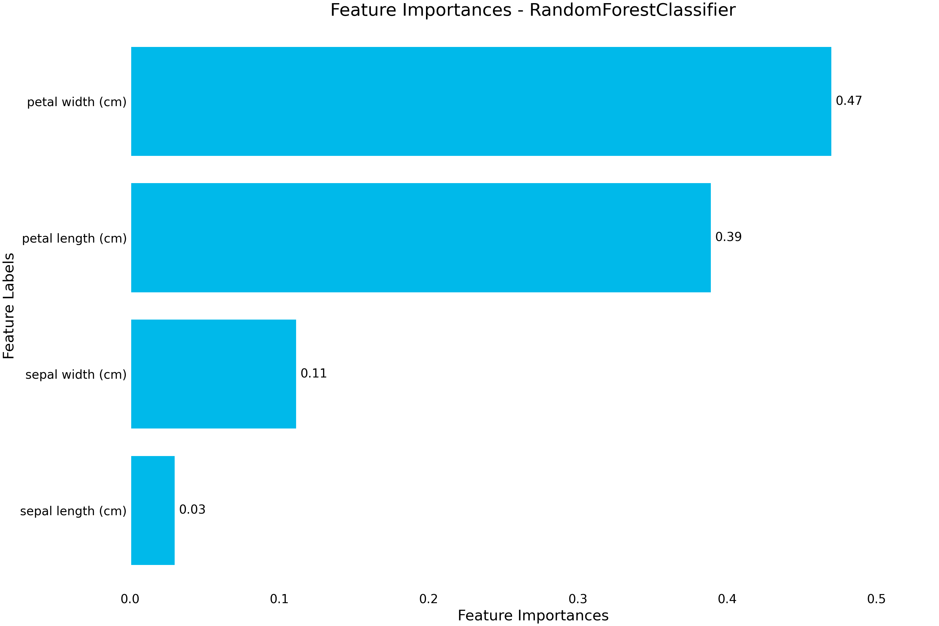
As the results are ordered by highest mean accuracy, we can select the first result and plot some diagnostic plots using the .plot accessor.

(Source code, png, hires.png, pdf)

We finish up by saving our best model to a local file, so we can reload that model later

>>> from ml_tooling.storage import FileStorage
>>>
>>> storage = FileStorage('./estimators')
>>> saved_path = best_model.save_estimator(storage)

If you are interested in more examples of how to use ml-tooling, please see the project notebooks.

Continue to Dataset